 Bifurcations
 Bifurcations

While there is a generally accepted precise definition for the term "first order differential equation'', this is not the case for the term "Bifurcation''. View "bifurcation" as a description of certain phenomena instead.
In a very crude way, we will say that a system undergoes a bifurcation if and only if the global behavior of a system, which depends on a parameter, changes when the parameter varies. Let us illustrate this through the population dynamics example. Indeed, consider the logistic equation describing a certain fish population
![]()
where P(t) is the population of the fish at time t. If we assume that the fish are harvested at a constant rate (for example), then we have to modify the differential equation to
![]()
where H > 0 is the constant harvesting rate. Here is a simple example of a real-world problem modeled by a differential equation involving a parameter (the constant rate H). Clearly, the fishermen will be happy if H is big, while ecologists will argue for a smaller H (in order to protect the fish population). What then is the ``optimal'' constant H (if such constant exists) which allows maximal harvesting without endangering the survival of the fish population?
First, let us look at the equilibria (or constant solutions) of this model. We must have
![]()
which gives
![]()
So
This is an example of what is meant by "bifurcation". As you see the number
of equilibria (or constant solutions) changes (from two to
zero) as the parameter H changes (from below 1/4 to above 1/4).
Note that this is just one form of bifurcation; there are other forms or
changes, which are also called bifurcations.
The Bifurcation Diagram
A very helpful way to illustrate bifurcations is through a Bifurcation Diagram. Again we will illustrate this tool via the harvesting example. Indeed consider the fish population modeled by the equation
![]()
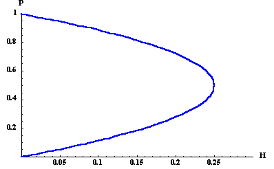
where H > 0 is the constant rate at which the fish are harvested. As we saw before depending on the number H we may have two, one, or no constant solutions. Let us draw this on a diagram with two axes
![]()
 |
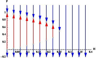
Let us add some vertical lines describing the phase lines. Indeed, for every number H, the vertical line given by H is the phase line associated with the differential equation
![]()
Recall that the phase line carries information on the nature of the
constant solutions (or equilibria) with respect to their
classification as sources, sinks, or nodes. This classification is
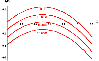
given by the sign of the function ![]() . The graph of
. The graph of
![]() for different values of H is given below
for different values of H is given below
 |
Putting everything together we get the following diagram (which is called the
bifurcation diagram)
 |
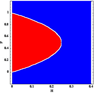
Instead of just drawing some phase lines, we will usually color the regions. The next picture illustrates this very nicely:
 |
Let us use this diagram to discuss the fate of the fish population as the parameter H increases. When H=0 (no fishing), the fish population tends to the carrying capacity P=1 which is a sink. If H increases but stays smaller than 0.25, then the fish population still tends to a new and smaller number
![]()
which is a also sink. When H is increased more and exceeds 0.25, then the differential equation has no equilibrium points (constant solutions). The fish population is decreasing and crosses the t-axis at finite time. This means that the fish population will vanish completely in finite time. Hence, in order to avoid such a catastrophic outcome, H needs to be slightly lower than 0.25, which is called the optimal harvesting rate. You should also keep in mind that a slightly smaller number will be a better choice than H=0.25 itself, since for H=0.25 the only equilibrium point P = 0.5 is not a sink (in fact, it is a node) and as soon as the population P falls below 0.5, we will again witness extinction in finite time.
The next animation illustrates the behavior of the solutions as H changes. The animation is based on the differential equation
 |
Click here for Exercises on bifurcation.

 S.O.S. MATHematics home page
Last Update 6-23-98